While working on Pitchy Ninja and Vexflow, I explored a variety of different techniques for pitch detection that would also work well in a browser. Although, I settled on a relatively well-known algorithm, the exploration took me down an interesting path -- I wondered if you could build neural networks to classify pitches, intervals, and chords in recorded audio.
Turns out the answer is yes. To all of them.
This post details some of the techniques I used to build a pitch-detection neural network. Although I focus on single-note pitch estimation, these methods seem to work well for multi-note chords too.
Pitch detection (also called fundamental frequency estimation) is not an exact science. What your brain perceives as pitch is a function of lots of different variables, from the physical materials that generate the sounds to your body's physiological structure.
One would presume that you can simply transform a signal to its frequency domain representation, and look at the peak frequencies. This would work for a sine wave, but as soon as you introduce any kind of timbre (e.g., when you sing, or play a note on a guitar), the spectrum is flooded with overtones and harmonic partials.
Here's a 33ms spectrogram of the note A4 (440hz) played on a piano. You can see a peak at 440hz, and another around 1760hz.

Here's the same A4 (440hz), but on a violin.

And here's a trumpet.

Notice how the thicker instruments have rich harmonic spectrums? These harmonics are what make them beautiful, and also what make pitch detection hard.
A lot of the well understood pitch estimation algorithms resort to transformations and heuristics which amplify the fundamental and cancel out the overtones. Some, more advanced techniques work on (kind of) fingerprinting timbres, and then attempting to correlate them with a signal.
For single tones, these techniques work well, but they do break down in their own unique ways. After all, they're heuristics that try to estimate human perception.
Deep convolutional networks have been winning image labeling challenges for nearly a decade, starting with AlexNet in 2012. The key insight in these architectures is that detecting objects require some level of locality in pattern recognition, i.e., learned features should be agnostic to translations, rotations, intensities, etc. Convolutional networks learn multiple layers of filters, each capturing some perceptual element.

For example, the bottom layer of an image recognition network might detect edges and curves, the next might detect simple shapes, and the next would detect objects, etc. Here's an example of extracted features from various layers (via DeepFeat.)

For audio feature extraction, time domain representations don't seem to be very useful to convnets. However, in the frequency domain, convnets learn features extremely well. Once networks start looking at spectrograms, all kinds of patterns start to emerge.
In the next few sections, we'll build a and train a simple convolutional network to detect fundamental frequencies across six octaves.
To do this well, we need data. Labeled. Lots of it! There are a few paths we can take:
Option 1: Go find a whole bunch of single-tone music online, slice it up into little bits, transcribe and label.
Option 2: Take out my trusty guitar, record, slice, and label. Then my keyboard, and my trumpet, and my clarinet. And maybe sing too. Ugh!
Option 3: Build synthetic samples with... code!
Since, you know, the ultimate programmer virtue is laziness, let's go with Option 3.
The goal is to build a model that performs well, and generalizes well, so we'll need to make sure that we account for enough of the variability in real audio as we can -- which means using a variety of instruments, velocities, effects, envelopes, and noise profiles.
With a good MIDI library, a patch bank, and some savvy, we can get this done. Here's what we need:
All of these are open-source and freely available. Download and install them before proceeding.
We start with picking a bunch of instruments encompassing a variety of different timbres and tonalities.
Pick the notes and octaves you want to be able to classify. I used all 12 tones between octaves 2 and 8 (and added some random detunings.) Here's a handy class to deal with note to MIDI value conversions.
The next section is where the meat of the synthesis happens. It does the following:
Finally, we use the Sample class to generate thousands of different 33ms long MIDI files, each playing a single note. The labels are part of the filename, and include the note, octave, frequency, and envelope component.
For this experiment, we're working with 44.1khz 16-bit samples, 33ms long -- which is about 14,500 data points per sample. We first downsample the audio to 16khz, yielding 5280 data points per sample.
The spectrogram will be generated via STFT, using a window size of 256, an overlap of 200, and a 1024 point FFT zero-padded on both sides. This yields one 513x90 pixel image per sample.
The 1024-point FFT also caps the resolution to about 19hz, which isn't perfect, but fine for distinguishing pitches.
Our network consists of 4 convolutional layers, with 64, 128, 128, and 256 filters respectively, which are then immediately downsampled with max-pooling layers. The input layer reshapes the input tensors by adding a channels dimension for Conv2D. We close out the model with two densely connected layers, and a final output node for the floating-point frequency.
To prevent overfitting, we regularize by aggressively adding dropout layers, including one right at the input which also doubles as an ad-hoc noise generator.
Although we use mean-squared-error as our loss function, it's the mean-absolute-error that we need to watch, since it's easier to reason about. Let's take a look at the model summary.

Wow, 12 million parameters! Feels like a lot for an experiment, but it turns out we can build a model in less than 10 minutes on a modern GPU. Let's start training.
After 100 epochs, we can achieve a validation MSE of 0.002, and a validation MAE of 0.03.

You may be wondering why the validation MAE is so much better than the training MAE. This is because of the aggressive dropout regularization. Dropout layers are only activated during training, not prediction.
These results are quite promising for an experiment! For classification problems, we could use confusion matrices to see where the models mispredict. For regression problems (like this one), we can explore the losses a bit more by plotting a graph of errors by pitch.
Already, we can see that the prediction errors are on the highest octaves. This is very likely due to our downsampling to 16khz, causing aliasing in the harmonics and confusing the model.
After discarding the last octave, we can take the mean of the prediction error, and what do we see?
Pretty much exactly the resolution of the FFT we used. It's very hard to do better given the inputs.
So, how does this perform in the wild? To answer this question, I recorded a few samples of myself playing single notes on the guitar, and pulled some youtube videos of various instruments and sliced them up for analysis. I also crossed my fingers and sacrificed a dozen goats.
As hoped, the predictions were right within the tolerances of the model. Try it yourself and let me know how it works out.
There's a few things we can do to improve what we have -- larger FFT and window sizes, higher sample rates, better data, etc. We can also turn this into a classification problem by using softmax at the bottom layer and training directly on musical pitches instead of frequencies.
This experiment was part of a whole suite of models I built for music recognition. In a future post I'll describe a more complex set of models I built to recognize roots, intervals, and 2-4 note chords.
Until then, hope you enjoyed this post. If you did, drop me a note at @11111110b.
All the source code for these experiments will be available on my Github page as soon as it's in slightly better shape.
Turns out the answer is yes. To all of them.
This post details some of the techniques I used to build a pitch-detection neural network. Although I focus on single-note pitch estimation, these methods seem to work well for multi-note chords too.
On Pitch Estimation
Pitch detection (also called fundamental frequency estimation) is not an exact science. What your brain perceives as pitch is a function of lots of different variables, from the physical materials that generate the sounds to your body's physiological structure.
One would presume that you can simply transform a signal to its frequency domain representation, and look at the peak frequencies. This would work for a sine wave, but as soon as you introduce any kind of timbre (e.g., when you sing, or play a note on a guitar), the spectrum is flooded with overtones and harmonic partials.
Here's a 33ms spectrogram of the note A4 (440hz) played on a piano. You can see a peak at 440hz, and another around 1760hz.

Here's the same A4 (440hz), but on a violin.

And here's a trumpet.

Notice how the thicker instruments have rich harmonic spectrums? These harmonics are what make them beautiful, and also what make pitch detection hard.
Estimation Techniques
A lot of the well understood pitch estimation algorithms resort to transformations and heuristics which amplify the fundamental and cancel out the overtones. Some, more advanced techniques work on (kind of) fingerprinting timbres, and then attempting to correlate them with a signal.
For single tones, these techniques work well, but they do break down in their own unique ways. After all, they're heuristics that try to estimate human perception.
Convolutional Networks
Deep convolutional networks have been winning image labeling challenges for nearly a decade, starting with AlexNet in 2012. The key insight in these architectures is that detecting objects require some level of locality in pattern recognition, i.e., learned features should be agnostic to translations, rotations, intensities, etc. Convolutional networks learn multiple layers of filters, each capturing some perceptual element.
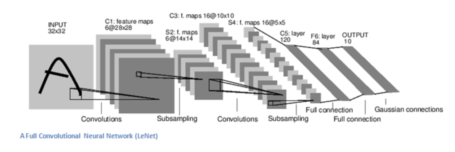
For example, the bottom layer of an image recognition network might detect edges and curves, the next might detect simple shapes, and the next would detect objects, etc. Here's an example of extracted features from various layers (via DeepFeat.)

Convolutional Networks for Audio
For audio feature extraction, time domain representations don't seem to be very useful to convnets. However, in the frequency domain, convnets learn features extremely well. Once networks start looking at spectrograms, all kinds of patterns start to emerge.
In the next few sections, we'll build a and train a simple convolutional network to detect fundamental frequencies across six octaves.
Getting Training Data
To do this well, we need data. Labeled. Lots of it! There are a few paths we can take:
Option 1: Go find a whole bunch of single-tone music online, slice it up into little bits, transcribe and label.
Option 2: Take out my trusty guitar, record, slice, and label. Then my keyboard, and my trumpet, and my clarinet. And maybe sing too. Ugh!
Option 3: Build synthetic samples with... code!
Since, you know, the ultimate programmer virtue is laziness, let's go with Option 3.
Tools of the Trade
The goal is to build a model that performs well, and generalizes well, so we'll need to make sure that we account for enough of the variability in real audio as we can -- which means using a variety of instruments, velocities, effects, envelopes, and noise profiles.
With a good MIDI library, a patch bank, and some savvy, we can get this done. Here's what we need:
- MIDIUtil - Python library to generate MIDI files.
- FluidSynth - Renders MIDI files to raw audio.
- GeneralUser GS - A bank of GM instrument patches for FluidSynth.
- sox - To post-process the audio (resample, normalize, etc.)
- scipy.io - For generating spectrograms
- Tensorflow - For building and training the models.
All of these are open-source and freely available. Download and install them before proceeding.
Synthesizing the Data
We start with picking a bunch of instruments encompassing a variety of different timbres and tonalities.
Pick the notes and octaves you want to be able to classify. I used all 12 tones between octaves 2 and 8 (and added some random detunings.) Here's a handy class to deal with note to MIDI value conversions.
The next section is where the meat of the synthesis happens. It does the following:
- Renders the MIDI files to raw audio (wav) using FluidSynth and a free GM sound font.
- Resamples to single-channel, unsigned 16-bit, at 44.1khz, normalized.
- Slices the sample up into its envelope components (attack, sustain, decay.)
- Detunes some of the samples to cover more of the harmonic surface.
Building the Network
Now that we have the training data, let's design the network.
I experimented with a variety of different architectures before I got here, starting with simple dense (non-convolution) networks with time-domain inputs, then moving on to one-dimensional LSTMs, then two-dimensional convolutional networks (convnets) with frequency-domain inputs.
As you can guess, the 2D networks with frequency-domain inputs worked significantly better. As soon as I got decent baseline performance with them, I focused on incrementally improving accuracy by reducing validation loss.
Model Inputs
The inputs to the network will be spectrograms, which are 2D images representing a slice of audio. The X-axis is usually time, and the Y-axis is frequency. They're great for visualizing audio spectrums, but also for more advanced audio analysis.
 |
| A Church Organ playing A4 (440hz) |
Spectrograms are typically generated with Short Time Fourier Transforms (STFTs). In short, the algorithm slides a window over the audio, running FFTs over the windowed data. Depending on the parameters of the STFT (and the associated FFTs), the precision of the detected frequencies can be tweaked to match the use case.
For this experiment, we're working with 44.1khz 16-bit samples, 33ms long -- which is about 14,500 data points per sample. We first downsample the audio to 16khz, yielding 5280 data points per sample.
The spectrogram will be generated via STFT, using a window size of 256, an overlap of 200, and a 1024 point FFT zero-padded on both sides. This yields one 513x90 pixel image per sample.
The 1024-point FFT also caps the resolution to about 19hz, which isn't perfect, but fine for distinguishing pitches.
The Network Model
Our network consists of 4 convolutional layers, with 64, 128, 128, and 256 filters respectively, which are then immediately downsampled with max-pooling layers. The input layer reshapes the input tensors by adding a channels dimension for Conv2D. We close out the model with two densely connected layers, and a final output node for the floating-point frequency.
To prevent overfitting, we regularize by aggressively adding dropout layers, including one right at the input which also doubles as an ad-hoc noise generator.

Wow, 12 million parameters! Feels like a lot for an experiment, but it turns out we can build a model in less than 10 minutes on a modern GPU. Let's start training.
After 100 epochs, we can achieve a validation MSE of 0.002, and a validation MAE of 0.03.

You may be wondering why the validation MAE is so much better than the training MAE. This is because of the aggressive dropout regularization. Dropout layers are only activated during training, not prediction.
These results are quite promising for an experiment! For classification problems, we could use confusion matrices to see where the models mispredict. For regression problems (like this one), we can explore the losses a bit more by plotting a graph of errors by pitch.
 |
| Prediction Errors by Pitch |
Already, we can see that the prediction errors are on the highest octaves. This is very likely due to our downsampling to 16khz, causing aliasing in the harmonics and confusing the model.
After discarding the last octave, we can take the mean of the prediction error, and what do we see?
np.mean(np.nan_to_num(errors_by_key[0:80]))
19.244542657486097Pretty much exactly the resolution of the FFT we used. It's very hard to do better given the inputs.
The Real Test
As hoped, the predictions were right within the tolerances of the model. Try it yourself and let me know how it works out.
Improvements and Variations
There's a few things we can do to improve what we have -- larger FFT and window sizes, higher sample rates, better data, etc. We can also turn this into a classification problem by using softmax at the bottom layer and training directly on musical pitches instead of frequencies.
This experiment was part of a whole suite of models I built for music recognition. In a future post I'll describe a more complex set of models I built to recognize roots, intervals, and 2-4 note chords.
Until then, hope you enjoyed this post. If you did, drop me a note at @11111110b.
All the source code for these experiments will be available on my Github page as soon as it's in slightly better shape.
No comments:
Post a Comment